We show an application of Gaussian isoperimetric inequality to machine learning. Specifically, we will take up the paper “Adversarial Examples Are a Natural Consequence of Test Error in Noise”. As its title states,the paper argues that “the existence of adversarial examples follows naturally from the fact that our models have nonzero test error in certain corrupted image distributions”, and this assertion is derived directly from Gaussian Isoperimetric Inequality. Note that the theorem of Gaussian Isoperimetric Inequality and its derivation are described in this post.
Curse of dimensionality
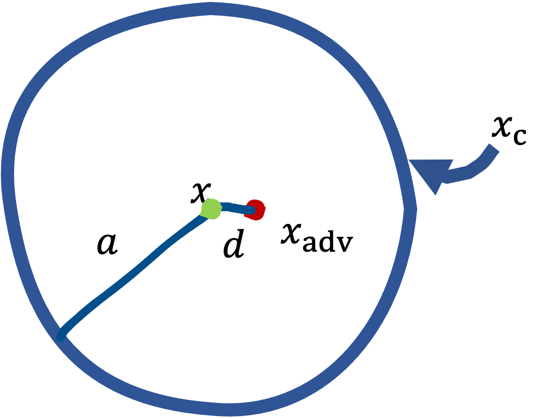
Corrupted images are generated by adding Gaussain noise sampled from $\mathcal{N}(0, \sigma^{2} \text{I})$ to the original input $x \in \mathbb{R}^{n}$, which is denoted by $x_{c}$. On the other hand, we denote the adversarial example generated based on $x$ as $x_{adv}$. The distance between each of them and $x$ is shown in the following intuitive picture.

$x_{c}$ are scattered over the circumference drawn in blue, and the radius of the circle, i.e., the distance between $x$ and $x_{c}$, is \[ a = \sigma \sqrt{n}. \] This is known as the Gaussian Annulus, and we can find very intuitive explanation in this paper. The other, the distance between $x_{adv}$ and $x$, which we denote as $d$, is the subject.
We consider common image classification tasks, for example, 10-class classification using CIFAR-10, and train a classifier $f$. Here we make the following assumption: the effect of the noise of $\mathcal{N}(0, \sigma^{2} \text{I})$ is faint to the human eyes, so one would consider $x_{c}$ to be the same as $x$. In other words, $f$ should predict the same class for $x_{c}$ as for $x$. Therefore, if the decision boundary that $f$ learns can be drawn so that it does not pass over the sphere on which $x_{c}$ are concentrated, the error rate will be almost zero. We denote the error rate of $f$ for $x_{c}$ by $\mu$. Considering a situation in which the decision boundary passes over the circle as shown in the figure below. In this case, the worst case is as shown in the red dot, and this can be $x_{adv}$.
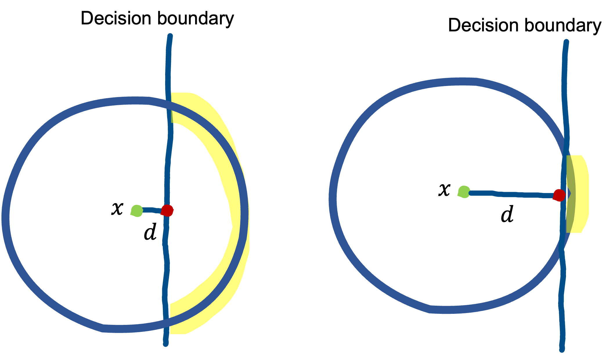
Suppose $\mu = 0.01$. This is the situation where only about $1\%$ of the points in the circle (though most of the points in fact are on the sphere of radius $a$ as mentioned) will be misclassified. What you may imagine in this situation is something like the figure on the left below, right?

However, the paper suggests that it would actually be like the figure on the right. What prevents our intuition from working well is the so-called curse of dimensionality. With the CDF of Gaussian $\Phi$, we show that \[ d = - \sigma \Phi(\mu). \] Remarkably, $d$ is independent of the dimensionality $n$, unlike $a$. We show that this form of $d$ is directly derived from Gaussian Isoperimetric Inequality.
Definition of robustness
Since the noise is generated by $\mathcal{N}(0, \sigma^{2} \text{I})$, we can view that the corrupted images $x_{c}$ are samples from the distribution $Q$ = $\mathcal{N}(x, \sigma^{2} \text{I})$. Let $E$ be the error set in which there exist the points for which the classifier $f$ makes an error prediction. Then, we difine corruption robustness as $P_{x \sim Q}(x \notin E )$, noting that the error rate we defined is written as \[ \mu = P_{x \sim Q}(x \in E ). \] Next, we define adversarial robustness. The shorter the distance from $x$ to the nearest point in $E$ (which we denote by $d(x,E)$), the more vulnerable it is to attacks. Thus, letting $P$ denote the distribution of natural images, the adversarial robustness is defined as $P_{x \sim P} (d(x,E) \gt \epsilon )$, the probability that a sample from $P$ is not within distance $\epsilon$ of some point in $E$. However, what we will use is not this one, but \[ P_{x \sim Q} (d(x,E) \gt \epsilon ). \] We will connect this probability to Gaussian measure $\gamma$.
Connecting to Gaussian measure
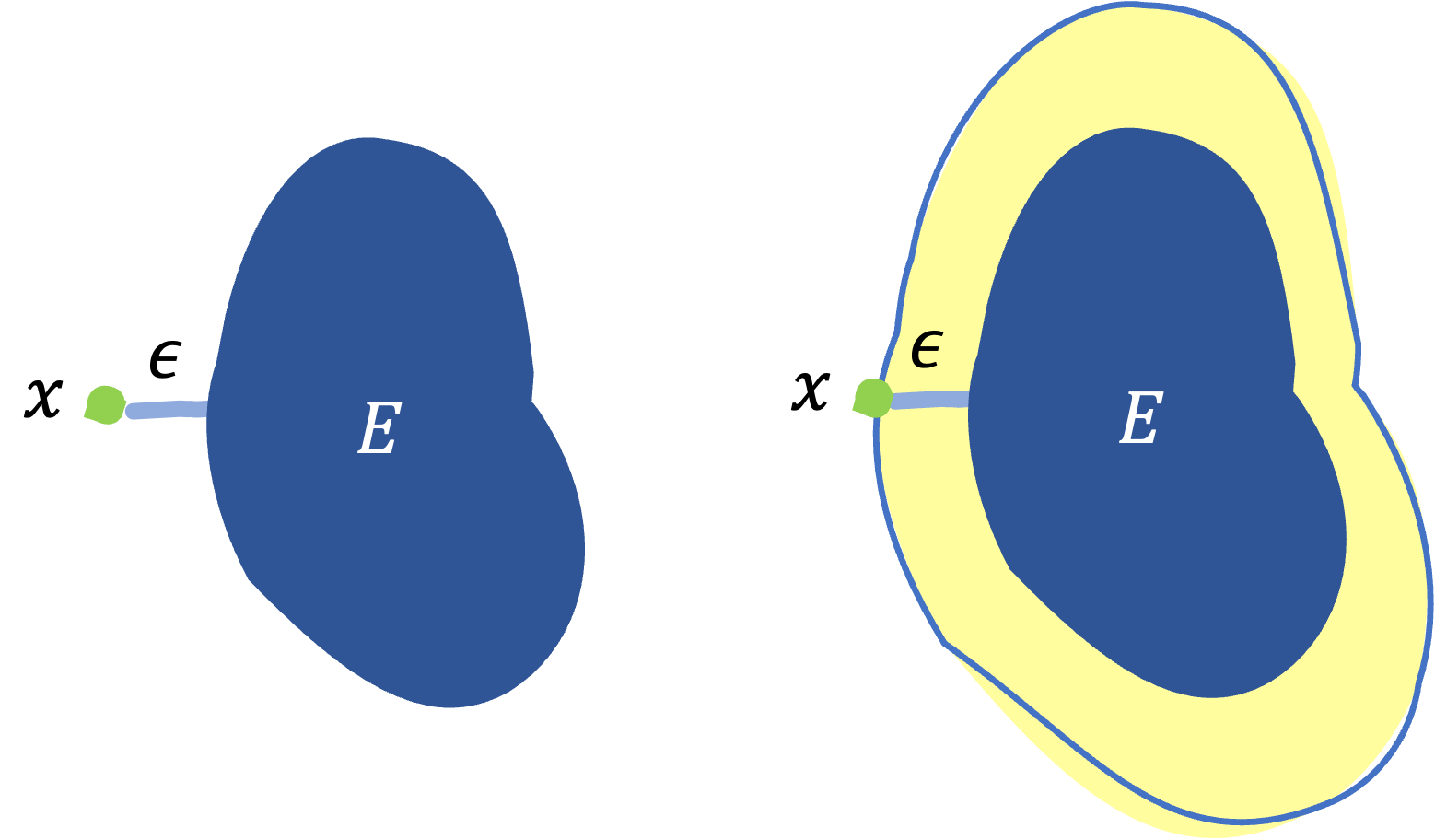
So far, we have been centering on $x$, but now we will shift our viewpoint to $E$. Let’s think of $E$ as a region rather than a set of datapoints and consider extending $E$ up to reach $x$, as the right one below.

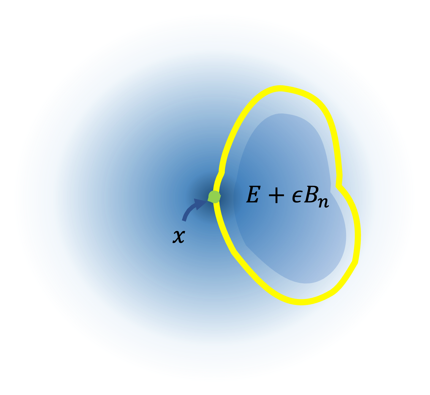
Suppose the thickness of the expansion is $\epsilon$, then we can view this as an $\epsilon$-extension, explained in this post, and the entire extended resion $E_{\epsilon}$ is represented as $E_{\epsilon} = E + \epsilon B_{n}$.

Placing $E_{\epsilon}$ in $n$-dimensional Ganssian distribution, $Q$, we can see the following connection: \[ P_{x \sim Q} (d(x,E) \gt \epsilon ) = \gamma(E + \epsilon B_{n}) \label{eq:1}\tag{1}. \] The RHS is obvious, just counting the measure of $E_{\epsilon}$. If we know that $d(x,E) \gt \epsilon $ includes not only $x$ in the region extending outside of $E$ by $\epsilon$, but also $x$ inside of $E$, this equality makes sense. In my opinion, this interpretation seems to be the most important point throughout.
Applying Gaussian Isoperimetric Inequality
Once we got Eq.$\,$($\ref{eq:1}$), all that remains is to apply Gaussian Isoperimetric Inequality, \[ \Phi^{-1} ( \gamma(E + \epsilon B_{n})) \geq \Phi^{-1} ( \gamma(E)) + \epsilon. \] Applying $\Phi^{-1}$ to the both terms of Eq.$\,$($\ref{eq:1}$), we obtain \[ \Phi^{-1} (P_{x \sim Q} (d(x,E) \gt \epsilon ) ) \geq \Phi^{-1} ( \gamma(E)) + \epsilon. \] With one last assumption, let us now consider the situation where $P_{x \sim Q} (d(x,E) \gt \epsilon ) = \frac{1}{2}$. It says that ralf of $x \sim Q$ generated are at a distance to $E$ shorter than $\epsilon$. Then, since $\Phi^{-1}(\frac{1}{2}) = 0$, we obtain \[ \epsilon = - \Phi^{-1}(\gamma(E)). \]